European Environment Agency (EEA) Air Quality Data#
The European Environment Agency (EEA) has a network of air quality monitoring stations across Europe. These stations record data for a number of pollutants, e.g. Particulate Matter 2.5 and Particulate Matter 10, and are placed in different environments to capture what is happening across both urban and rural areas. To learn more about the stations and look up station codes, explore the European Air Quality Index map.
In the air quality directive (2008/EC/50), the EU has set two limit values for particulate matter (PM10) for the protection of human health: the PM10 daily mean value may not exceed 50 micrograms per cubic metre (µg/m3) more than 35 times in a year and the PM10 annual mean value may not exceed 40 micrograms per cubic metre (µg/m3). (Source)
As for PM2.5, no daily limit has been set by the EU, but the World Health Organisation’s daily limit is 25 micrograms per cubic metre (µg/m3). Read more here.
Basic facts
Spatial coverage: Observation stations across Europe
Temporal resolution: daily aggregates
Data format: csv
How to access the data
The EEA air quality data is available for download via the EEA Air Quality Portal.
The Python library airbase allows you to download all EEA Air Quality data for a country at once. You can specify which pollutant, country and time period you want to download. Read more about the library here.
The first part of this notebook (1 - Download EEA Air Quality data for specific pollutants and countries) shows you how to request EEA Air Quality data with the library airbase.
Load required libraries
import numpy as np
import pandas as pd
import airbase

import matplotlib.pyplot as plt
Optional: Download EEA Air Quality data for specific pollutants and countries#
The Python library airbase allows you to download all EEA Air Quality data for a country at once. You can specify which pollutant, country and time period you want to download. Read more about the library here. Due to the large file sizes, it is recommended to download data for each country and pollutant (PM10 and PM2.5) separately. We have predownloaded data for the station Palma de Mallorca, Spain for you.
The first step is to store the airbase client in a variable called client.
client = airbase.AirbaseClient()
Next, we define a download request by stating which country, pollutant and year we want the data from. The abbreviation for Spain is "ES" and the pollutant is "PM10". We only want data from 2024, so we specify both, the year_from and year_to as 2024.
By using the function download_to_file(), all the 490 resulting CSVs are concatenated into a single CSV file called ES_PM10_2024.csv. Each CSV contains data from a single station. It is recommended to download all the data for a country into one CSV to make it easier to search for a station using the station code. You are able to change the file name to anything you wish. We also specify where the data should be stored by stating the file path "../../eodata/2_observations/eea/ES/ES_PM10_2024.csv".
We have commented out the code as these data have already been downloaded for you.
#r = client.request(country=["ES"], pl=["PM10"], year_from=2024, year_to=2024)
#r.download_to_file("../../eodata/2_observations/eea/ES/ES_PM10_2024.csv")
Next, we download the PM2.5 data for Spain and store it in a CSV called ES_PM2pt5_2024.csv. You will notice that there are fewer stations that collect PM2.5 data, just 226.
#r = client.request(country=["ES"], pl=["PM2.5"], year_from=2024, year_to=2024)
#r.download_to_file("../../eodata/2_observations/eea/ES/ES_PM10_2024.csv")
Read the observation data with pandas#
For this exercise, we will focus on the Palma de Mallorca Station, Spain.
The EEA air quality station in Palma de Mallorca has the code ES2097A. You can find the file in the folder ../../eodata/2_observations/eea/ES/palma/. You can read csv files with the function read_table() from the Python library pandas. We can set additonal keyword arguments that allow us to specify the columns and rows of interest:
delimiter: specify the delimiter in the text file, e.g. commaheader: specify the index of the row that shall be set as header.index_col: specify the index of the column that shall be set as indexlow_memory: this is set toFalsein this case to avoid mixed type interference
Because the data is stored in a comma-separated values file, the delimiter is set to ,. The first row of the file contains the header information, thus we set the header value to [0]. Finally, we set the index column to be the 5th column in the file, which is the AirQualityStationEoICode.
You see below that the resulting dataframe has 3601 rows and 16 columns.
df = pd.read_table('../../eodata/2_observations/eea/ES/palma/ES_5_68795_2024_timeseries.csv', delimiter=',', header=[0], index_col=4, low_memory=False)
df
| Countrycode | Namespace | AirQualityNetwork | AirQualityStation | SamplingPoint | SamplingProcess | Sample | AirPollutant | AirPollutantCode | AveragingTime | Concentration | UnitOfMeasurement | DatetimeBegin | DatetimeEnd | Validity | Verification | |
|---|---|---|---|---|---|---|---|---|---|---|---|---|---|---|---|---|
| AirQualityStationEoICode | ||||||||||||||||
| ES2097A | ES | ES.BDCA.AQD | NET_ES205A | STA_ES2097A | SP_35016014_10_49 | SPP_35016014_10_49.1 | SAM_35016014_10_49 | PM10 | http://dd.eionet.europa.eu/vocabulary/aq/pollu... | hour | 32.0 | µg/m3 | 2024-01-01 01:00:00 +01:00 | 2024-01-01 02:00:00 +01:00 | 1 | 3 |
| ES2097A | ES | ES.BDCA.AQD | NET_ES205A | STA_ES2097A | SP_35016014_10_49 | SPP_35016014_10_49.1 | SAM_35016014_10_49 | PM10 | http://dd.eionet.europa.eu/vocabulary/aq/pollu... | hour | 42.0 | µg/m3 | 2024-01-01 02:00:00 +01:00 | 2024-01-01 03:00:00 +01:00 | 1 | 3 |
| ES2097A | ES | ES.BDCA.AQD | NET_ES205A | STA_ES2097A | SP_35016014_10_49 | SPP_35016014_10_49.1 | SAM_35016014_10_49 | PM10 | http://dd.eionet.europa.eu/vocabulary/aq/pollu... | hour | 30.0 | µg/m3 | 2024-01-01 04:00:00 +01:00 | 2024-01-01 05:00:00 +01:00 | 1 | 3 |
| ES2097A | ES | ES.BDCA.AQD | NET_ES205A | STA_ES2097A | SP_35016014_10_49 | SPP_35016014_10_49.1 | SAM_35016014_10_49 | PM10 | http://dd.eionet.europa.eu/vocabulary/aq/pollu... | hour | 25.0 | µg/m3 | 2024-01-01 06:00:00 +01:00 | 2024-01-01 07:00:00 +01:00 | 1 | 3 |
| ES2097A | ES | ES.BDCA.AQD | NET_ES205A | STA_ES2097A | SP_35016014_10_49 | SPP_35016014_10_49.1 | SAM_35016014_10_49 | PM10 | http://dd.eionet.europa.eu/vocabulary/aq/pollu... | hour | 24.0 | µg/m3 | 2024-01-01 07:00:00 +01:00 | 2024-01-01 08:00:00 +01:00 | 1 | 3 |
| ... | ... | ... | ... | ... | ... | ... | ... | ... | ... | ... | ... | ... | ... | ... | ... | ... |
| ES2097A | ES | ES.BDCA.AQD | NET_ES205A | STA_ES2097A | SP_35016014_10_49 | SPP_35016014_10_49.1 | SAM_35016014_10_49 | PM10 | http://dd.eionet.europa.eu/vocabulary/aq/pollu... | hour | NaN | µg/m3 | 2024-05-29 13:00:00 +01:00 | 2024-05-29 14:00:00 +01:00 | -1 | 3 |
| ES2097A | ES | ES.BDCA.AQD | NET_ES205A | STA_ES2097A | SP_35016014_10_49 | SPP_35016014_10_49.1 | SAM_35016014_10_49 | PM10 | http://dd.eionet.europa.eu/vocabulary/aq/pollu... | hour | NaN | µg/m3 | 2024-05-29 14:00:00 +01:00 | 2024-05-29 15:00:00 +01:00 | -1 | 3 |
| ES2097A | ES | ES.BDCA.AQD | NET_ES205A | STA_ES2097A | SP_35016014_10_49 | SPP_35016014_10_49.1 | SAM_35016014_10_49 | PM10 | http://dd.eionet.europa.eu/vocabulary/aq/pollu... | hour | 16.0 | µg/m3 | 2024-05-29 21:00:00 +01:00 | 2024-05-29 22:00:00 +01:00 | 1 | 3 |
| ES2097A | ES | ES.BDCA.AQD | NET_ES205A | STA_ES2097A | SP_35016014_10_49 | SPP_35016014_10_49.1 | SAM_35016014_10_49 | PM10 | http://dd.eionet.europa.eu/vocabulary/aq/pollu... | hour | 14.0 | µg/m3 | 2024-05-29 22:00:00 +01:00 | 2024-05-29 23:00:00 +01:00 | 1 | 3 |
| ES2097A | ES | ES.BDCA.AQD | NET_ES205A | STA_ES2097A | SP_35016014_10_49 | SPP_35016014_10_49.1 | SAM_35016014_10_49 | PM10 | http://dd.eionet.europa.eu/vocabulary/aq/pollu... | hour | NaN | µg/m3 | 2024-05-29 23:00:00 +01:00 | 2024-05-30 00:00:00 +01:00 | -1 | 3 |
3601 rows × 16 columns
Then, we select only columns that contain data of interest, the Concentration of PM10 and DatetimeBegin, and reorder them so that DatetimeBegin is the first column.
# select columns by name
df = df.filter(items=['Concentration','DatetimeBegin'])

# Reset DataFrame with columns in desired order
df = df[['DatetimeBegin','Concentration']]
df
| DatetimeBegin | Concentration | |
|---|---|---|
| AirQualityStationEoICode | ||
| ES2097A | 2024-01-01 01:00:00 +01:00 | 32.0 |
| ES2097A | 2024-01-01 02:00:00 +01:00 | 42.0 |
| ES2097A | 2024-01-01 04:00:00 +01:00 | 30.0 |
| ES2097A | 2024-01-01 06:00:00 +01:00 | 25.0 |
| ES2097A | 2024-01-01 07:00:00 +01:00 | 24.0 |
| ... | ... | ... |
| ES2097A | 2024-05-29 13:00:00 +01:00 | NaN |
| ES2097A | 2024-05-29 14:00:00 +01:00 | NaN |
| ES2097A | 2024-05-29 21:00:00 +01:00 | 16.0 |
| ES2097A | 2024-05-29 22:00:00 +01:00 | 14.0 |
| ES2097A | 2024-05-29 23:00:00 +01:00 | NaN |
3601 rows × 2 columns
Now, let us change the index column to the start time column DatetimeBegin by using set_index(). Then we will resample the hourly data into daily data using .resample(), passing in D for day, and .mean() to calculate the mean.
Finally, in order to differentiate the data later on, we rename the column from Concentration to PM10.
# Set date column as index
df = df.set_index('DatetimeBegin')

# Converting the Index to a DatetimeIndex
df.index = pd.to_datetime(df.index)

# Resample hourly data to daily mean of PM10
pm10_daily = df.resample('D').mean()

# Rename Concentration column
pm10_daily.rename(columns={'Concentration': 'PM10'}, inplace=True)
pm10_daily
| PM10 | |
|---|---|
| DatetimeBegin | |
| 2024-01-01 00:00:00+01:00 | 31.666667 |
| 2024-01-02 00:00:00+01:00 | 25.333333 |
| 2024-01-03 00:00:00+01:00 | 21.208333 |
| 2024-01-04 00:00:00+01:00 | 15.833333 |
| 2024-01-05 00:00:00+01:00 | 3.708333 |
| ... | ... |
| 2024-05-26 00:00:00+01:00 | 12.166667 |
| 2024-05-27 00:00:00+01:00 | 13.833333 |
| 2024-05-28 00:00:00+01:00 | 16.541667 |
| 2024-05-29 00:00:00+01:00 | 15.647059 |
| 2024-05-30 00:00:00+01:00 | NaN |
151 rows × 1 columns
Now, let us repeat all the above steps for the PM2.5 data for the same station.
df2 = pd.read_table('../../eodata/2_observations/eea/ES/palma/ES_6001_68800_2024_timeseries.csv', delimiter=',', header=[0], index_col=4, low_memory=False)

# select columns by name
df2 = df2.filter(items=['Concentration','DatetimeBegin'])

# Reset DataFrame with columns in desired order
df2 = df2[['DatetimeBegin','Concentration']]

# Set date column as index
df2 = df2.set_index('DatetimeBegin')

# Converting the Index to a DatetimeIndex
df2.index = pd.to_datetime(df2.index)

# Resample hourly data to daily mean of PM2.5
pm2pt5_daily = df2.resample('D').mean()

# Rename Concentration column
pm2pt5_daily.rename(columns={'Concentration': 'PM2.5'}, inplace=True)
pm2pt5_daily
| PM2.5 | |
|---|---|
| DatetimeBegin | |
| 2024-01-01 00:00:00+01:00 | 12.125000 |
| 2024-01-02 00:00:00+01:00 | 8.833333 |
| 2024-01-03 00:00:00+01:00 | 7.875000 |
| 2024-01-04 00:00:00+01:00 | 6.041667 |
| 2024-01-05 00:00:00+01:00 | 1.833333 |
| ... | ... |
| 2024-05-26 00:00:00+01:00 | 7.208333 |
| 2024-05-27 00:00:00+01:00 | 6.750000 |
| 2024-05-28 00:00:00+01:00 | 8.083333 |
| 2024-05-29 00:00:00+01:00 | 7.352941 |
| 2024-05-30 00:00:00+01:00 | NaN |
151 rows × 1 columns
Because we are interested in plotting only data for April 2024, we have to filter both data frames further. Using .index.to_series() enables us to turn the DatetimeIndex into a series. We then can pass the start date of 2024-04-01 and the end date of 2024-04-28 to the .between() method to filter this series to only April 2024.
pm10_Apr2024 = pm10_daily[pm10_daily.index.to_series().between('2024-04-01', '2024-04-30')]
pm10_Apr2024
| PM10 | |
|---|---|
| DatetimeBegin | |
| 2024-04-01 00:00:00+01:00 | 16.304348 |
| 2024-04-02 00:00:00+01:00 | 9.041667 |
| 2024-04-03 00:00:00+01:00 | 8.043478 |
| 2024-04-04 00:00:00+01:00 | 7.636364 |
| 2024-04-05 00:00:00+01:00 | 12.166667 |
| 2024-04-06 00:00:00+01:00 | 11.458333 |
| 2024-04-07 00:00:00+01:00 | 16.000000 |
| 2024-04-08 00:00:00+01:00 | 14.125000 |
| 2024-04-09 00:00:00+01:00 | 25.625000 |
| 2024-04-10 00:00:00+01:00 | 46.291667 |
| 2024-04-11 00:00:00+01:00 | 92.083333 |
| 2024-04-12 00:00:00+01:00 | 31.625000 |
| 2024-04-13 00:00:00+01:00 | 28.416667 |
| 2024-04-14 00:00:00+01:00 | 37.000000 |
| 2024-04-15 00:00:00+01:00 | 101.500000 |
| 2024-04-16 00:00:00+01:00 | 80.416667 |
| 2024-04-17 00:00:00+01:00 | 26.272727 |
| 2024-04-18 00:00:00+01:00 | 39.125000 |
| 2024-04-19 00:00:00+01:00 | 48.875000 |
| 2024-04-20 00:00:00+01:00 | 20.750000 |
| 2024-04-21 00:00:00+01:00 | 14.166667 |
| 2024-04-22 00:00:00+01:00 | 23.458333 |
| 2024-04-23 00:00:00+01:00 | 23.750000 |
| 2024-04-24 00:00:00+01:00 | 23.500000 |
| 2024-04-25 00:00:00+01:00 | 24.625000 |
| 2024-04-26 00:00:00+01:00 | 17.375000 |
| 2024-04-27 00:00:00+01:00 | 10.333333 |
| 2024-04-28 00:00:00+01:00 | 11.125000 |
| 2024-04-29 00:00:00+01:00 | 5.523810 |
| 2024-04-30 00:00:00+01:00 | 6.875000 |
pm2pt5_Apr2024 = pm2pt5_daily[pm2pt5_daily.index.to_series().between('2024-04-01', '2024-04-30')]
pm2pt5_Apr2024
| PM2.5 | |
|---|---|
| DatetimeBegin | |
| 2024-04-01 00:00:00+01:00 | 7.260870 |
| 2024-04-02 00:00:00+01:00 | 4.125000 |
| 2024-04-03 00:00:00+01:00 | 3.521739 |
| 2024-04-04 00:00:00+01:00 | 3.681818 |
| 2024-04-05 00:00:00+01:00 | 5.083333 |
| 2024-04-06 00:00:00+01:00 | 5.208333 |
| 2024-04-07 00:00:00+01:00 | 7.041667 |
| 2024-04-08 00:00:00+01:00 | 6.583333 |
| 2024-04-09 00:00:00+01:00 | 11.833333 |
| 2024-04-10 00:00:00+01:00 | 20.208333 |
| 2024-04-11 00:00:00+01:00 | 27.458333 |
| 2024-04-12 00:00:00+01:00 | 12.500000 |
| 2024-04-13 00:00:00+01:00 | 14.541667 |
| 2024-04-14 00:00:00+01:00 | 16.833333 |
| 2024-04-15 00:00:00+01:00 | 29.916667 |
| 2024-04-16 00:00:00+01:00 | 25.541667 |
| 2024-04-17 00:00:00+01:00 | 12.681818 |
| 2024-04-18 00:00:00+01:00 | 16.500000 |
| 2024-04-19 00:00:00+01:00 | 17.583333 |
| 2024-04-20 00:00:00+01:00 | 8.458333 |
| 2024-04-21 00:00:00+01:00 | 6.041667 |
| 2024-04-22 00:00:00+01:00 | 10.750000 |
| 2024-04-23 00:00:00+01:00 | 10.875000 |
| 2024-04-24 00:00:00+01:00 | 11.500000 |
| 2024-04-25 00:00:00+01:00 | 10.583333 |
| 2024-04-26 00:00:00+01:00 | 7.666667 |
| 2024-04-27 00:00:00+01:00 | 4.250000 |
| 2024-04-28 00:00:00+01:00 | 4.791667 |
| 2024-04-29 00:00:00+01:00 | 2.523810 |
| 2024-04-30 00:00:00+01:00 | 3.000000 |
Visualize daily EEA PM10 and EEA PM2.5 at Palma de Mallorca, Spain for April 2024#
The next step is to visualize all points of PM10 and PM2.5 at Palma de Mallorca, Spain for April 2024.
You can use the built-in plot() function of the pandas library to define a line plot. With the filter function, you can select the dataframe columns you wish to visualize. The visualisation code below consists of five main parts:
Initiate a matplotlib figureDefine a line plot with the built-in plot function of the pandas librarySet title and axes label informationFormat axes ticksAdd additional features, such as a grid or legend
# Initiate a matplotlib figure
fig = plt.figure(figsize=(20,10))
ax = plt.axes()

# Select pandas dataframe columns and define a line plot for PM10 and PM2.5 each
pm10_Apr2024.filter(['PM10']).plot(ax=ax, style='o-', label='PM10')
pm2pt5_Apr2024.filter(['PM2.5']).plot(ax=ax, style='o-',label='PM2.5')
plt.axhline(y=50, color='r', linestyle='dotted', label='PM10 daily limit')

# Set title and axes lable information
plt.title('\nPM2.5 and PM10 for April 2024 - Palma de Mallorca, Spain', fontsize=20, pad=20)
plt.ylabel('Particulate matter in micrograms per cubic metre (µg/m3)\n', fontsize=16)

plt.xlabel('Day', fontsize=16)

# Format the axes ticks
plt.xticks(fontsize=16)
plt.yticks(fontsize=16)

# Set major ticks on the y-axis every 10, minor ticks every 5
major_ticks = np.arange(0, 101, 10)
minor_ticks = np.arange(0, 101, 5)
ax.set_yticks(major_ticks)
ax.set_yticks(minor_ticks, minor=True)

# Use different settings for the grids
ax.grid(which='minor', alpha=0.2)
ax.grid(which='major', alpha=0.8)

# Add additionally a legend and grid to the plot
plt.legend(fontsize=16,loc=0)
plt.show()
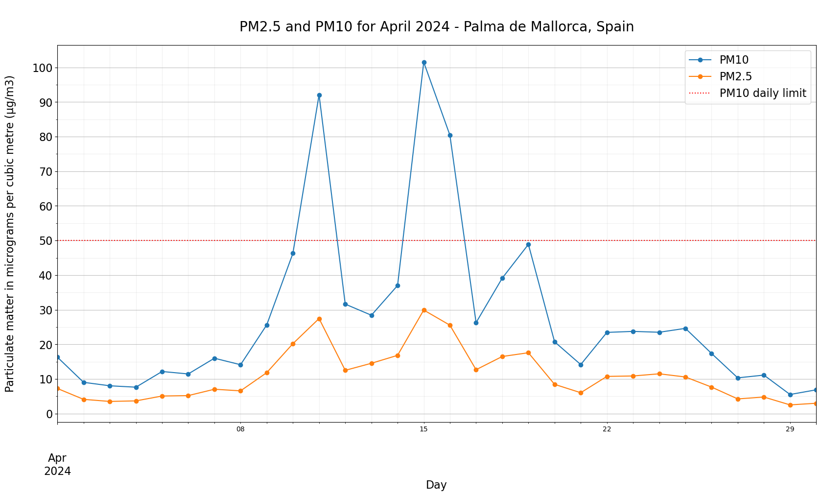
The plot shows you that the PM10 guidelines of 50µg/m3 set by the EU were exceeded multiple times between 10th and 17th April 2024.